40 excel scatter chart data labels
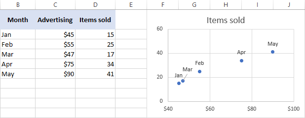
How to Make Route Map in Excel (2 Simple Ways) - ExcelDemy In the Insert tab, select the drop-down arrow of Insert Scatter (X, Y) or Bubble Chart and choose the Scatter with Smooth Lines and Markers option from the Charts group. The chart will appear in front of you. After that, uncheck all the Chart Elements except the Data Labels. You can see that the dots are showing the value of the Y-axis. Exp19_excel_ch03_ml2_grades | Computer Science homework help You want to add data labels to indicate the category and percentage of the class that earned each letter grade Add centered data labels. Select data label options to display Percentage and Category Name in the Inside End position. Remove the Values data labels. Apply 20-pt size and apply Black, Text 1 font color to the data labels.
Excel Units - A B C D | StudyHippo.com A scatter chart ____. answer. compares trends over uneven time or measurement intervals. ... You can change the ____ of labels and values in cells to be left, right, or center. answer. alignment. ... Text annotations are ____ that you can add to further describe the data in your chart. answer. labels. question. The default border color around a ...

Excel scatter chart data labels
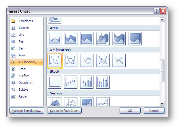
How to Refresh Chart in Excel (2 Effective Ways) - ExcelDemy Let's follow the instructions below to refresh a chart! Step 1: First of all, select the data range. From our dataset, we will select B4 to D10 for the convenience of our work. Hence, from your Insert tab, go to, Insert → Tables → Table As a result, a Create Table dialog box will appear in front of you. From the Create Table dialog box, press OK. support.microsoft.com › en-us › topicHow to use a macro to add labels to data points in an xy ... The labels and values must be laid out in exactly the format described in this article. (The upper-left cell does not have to be cell A1.) To attach text labels to data points in an xy (scatter) chart, follow these steps: On the worksheet that contains the sample data, select the cell range B1:C6. How to create a magic quadrant chart in Excel - Data Cornering Here are steps on how to create a quadrant chart in Excel, but you can download the result below. 1. Select columns with X and Y parameters and insert a scatter chart. 2. Select the horizontal axis of the axis and press shortcut Ctrl + 1. 3. Set the minimum, maximum, and position where the vertical axis crosses.
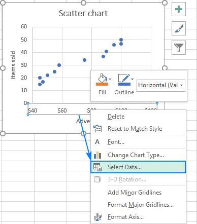
Excel scatter chart data labels. How to Create a Matrix Chart in Excel (2 Common Types) Select the range of values ( C4:D8) and then go to the Insert Tab >> Charts Group >> Insert Scatter (X, Y) or Bubble Chart Dropdown >> Scatter Option. After that, the following graph will appear. Now, we have to set the upper bound and lower bound limits of the X-axis and Y-axis. Firstly, select the X-axis label and then Right-click here. › add-vertical-line-excel-chartAdd vertical line to Excel chart: scatter plot, bar and line ... May 15, 2019 · Add vertical line to Excel scatter chart; Insert vertical line in Excel bar chart; Add vertical line to line chart; How to add vertical line to scatter plot. To highlight an important data point in a scatter chart and clearly define its position on the x-axis (or both x and y axes), you can create a vertical line for that specific data point ... Excel: How To Convert Data Into A Chart/Graph - Rowan University 7: To add axis titles, data labels, legend, trendline, and more, click the graph you just created. A new tab titled "Chart design" should appear. In the upper menu of that tab, you should see a section called "add chart element." 8: In "add chart element," you can customize your graph to your liking . STEP 9: Don't forget to save your work! Scatter chart - two data points not in date order One more workaround is to use line chart in place of scatter chart, and not use the line color but just the marker color, and sort by date. It works fine even with legend, but you need to specify legend colors manually while publishing the report. Hope it helps. View solution in original post Message 10 of 11 51 Views 1 Reply All forum topics
peltiertech.com › multiple-time-series-excel-chartMultiple Time Series in an Excel Chart - Peltier Tech Aug 12, 2016 · Start by selecting the monthly data set, and inserting a line chart. Excel has detected the dates and applied a Date Scale, with a spacing of 1 month and base units of 1 month (below left). Select and copy the weekly data set, select the chart, and use Paste Special to add the data to the chart (below right). A Beginner's Guide on How to Plot a Graph in Excel Firstly, select the cells that have the data you want to use in your graph by clicking and dragging across the cells. Secondly, once the text is highlighted, you can select a graph. Click the Insert tab and click your chart or graph you wish to use. Now you have your graph. Finally, customize your graph for aesthetics and convenience. How to make a 3 Axis Graph using Excel? - GeeksforGeeks To create a 3 axis graph follow the following steps: Step 1: Select table B3:E12.Then go to Insert Tab, and select the Scatter with Chart Lines and Marker Chart.. Step 2: A Line chart with a primary axis will be created. Step 3: The primary axis of the chart will be Temperature, the secondary axis will be Pressure and the third axis will be Volume.So, to create the third axis duplicate this ... Google Charts Hide Axis Labels - fpb.politecnico.lucca.it for stacked bar charts, excel 2010 allows you to add data labels only to the individual components of the stacked bar chart set_position (" center ") # most the bottom axis to the center ax of oil reserves' as data values along y-axis to create labels consisting only of numbers, enclose the numbers in straight quotation marks to create labels …
› documents › excelHow to display text labels in the X-axis of scatter chart in ... Actually, there is no way that can display text labels in the X-axis of scatter chart in Excel, but we can create a line chart and make it look like a scatter chart. 1. Select the data you use, and click Insert > Insert Line & Area Chart > Line with Markers to select a line chart. See screenshot: 2. Then right click on the line in the chart to ... How to Hack Excel — and Add Totals to the Tops of Stacked Column Charts It was done by understanding how scatter plots are built. Scatter plots place your data in certain positions, based on the x,y coordinates provided. You could use that to prepare the data for a scatter plot that looks like the US, then add the data, add hexagons, and so on. Since someone already did that, you can simply read up on their work. Excel 365 - Linear Trendline Equation Wrong (negative slope is ... The chart of the series reflects the new data (upward trend). But the trendline label is not changed. It still has the trendline equation with the negative slope.-----BTW, when I copy "bad chart" after editing the trendline label (i.e. it is now in the bad state), "bad chart (copy)" retains the bad state. A Step-by-Step Guide on How to Make a Graph in Excel For labels on the horizontal axis labels, you may select confirmed cases, deaths, recovered, and active cases, and depict them on the chart. After specifying the entries, click on OK. This will display the pie chart on your window. You can click on the icons next to the chart to add your finishing touches to it.
INLS161-001 Spring 2015 Information Tools | data display
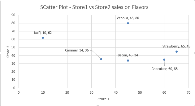
excel - How to getting text labels to show up in scatter chart - Stack ... How to getting text labels to show up in scatter chart. I want text labels for my scatter plot that is connected with points in the graph. my data is like this. The chart removes the labels and places numbers. How do I get the text labels back?
Add Custom Labels to x-y Scatter plot in Excel - DataScience Made Simple
Probability Chart in Excel | Microsoft Excel Tips | Excel Tutorial ... Double click on the small square in the right bottom corner of the cell. Label Column B Expected. Click on B2 (1), and type =NORM.S.INV (D2) (2) Double click on the small square showing in the result from previous step. Highlight A2-B8 (1), click on insert (2), scatter chart (3), and choose desired chart (4) to plot normal distribution chart.

Add Labels to Outliers in Excel Scatter Charts – System Secrets
Multiple How To Make Scatter Excel With Plot Data In A Sets How to Run a Multiple Regression in Excel Important features of the data are easy to discern (central tendency, bimodality, skew), and they afford easy comparisons between subsets To add data labels to scatter plot in Excel, follow the steps below: Click on the chart make sure that Excel is using a date-based axis How to Merge Sheets in Excel How to Merge Sheets in Excel.

Scatter Chart in Excel
support.microsoft.com › en-us › topicPresent your data in a scatter chart or a line chart Scatter charts and line charts look very similar, especially when a scatter chart is displayed with connecting lines. However, the way each of these chart types plots data along the horizontal axis (also known as the x-axis) and the vertical axis (also known as the y-axis) is very different.

Creating 3-D Scatter Plots - MATLAB & Simulink - MathWorks América Latina
I couldn't see the graph in excel, plot area. As I As I explained, I enter the data in excel. select them and - Answered by a verified Microsoft Office Technician. ... I have a excel point graph where some of the data point labels do not appear on the graph. ... A pie chart II) An exploded pie chart III) An area chart IV) An X Y (scatter) chart V) ...
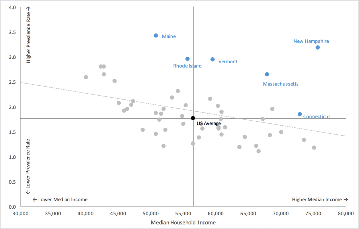
Excel Scatterplot with Custom Annotation - PolicyViz
Peltier Tech Excel Charts and Programming Blog This works for the chart title, axis titles, data labels, and textboxes and other shapes that contain text. ... If we plot XY scatter data on the chart, Excel treats the categories as if the first category is at X=1, the second at X=2, and so on. For the XY scatter data, we can consider the axis as a continuous numerical scale starting at the ...
3d scatter plot for MS Excel
Excel Datatemplate - 18 images - microsoft excel data lists, creating ... Excel Datatemplate. Here are a number of highest rated Excel Datatemplate pictures upon internet. We identified it from honorable source. Its submitted by executive in the best field. We say you will this nice of Excel Datatemplate graphic could possibly be the most trending topic following we share it in google improvement or facebook.
How to make a scatter plot in Excel
How to Map Data in Excel (2 Easy Methods) - ExcelDemy For demonstration purposes, we are going to use the following dataset. Let's walk through the following steps. 📌 Steps: First of all, select the range of the dataset as shown below. Next, go to the Insert tab from your ribbon. Then, select Maps from the Tours group. Now, select the Open 3D Maps icon from the drop-down list

Column Chart in Excel - EASY Excel Tutorial
12 Best Line Graph Maker Tools For Creating Stunning Line Graphs [2022 ... Plotly Chart Studio provides the solution for creating the graphs online. The graph can be created by importing the data from Excel, CSV, and SQL. It helps in creating many types of graphs and charts like bar charts, box plots, line graphs, dot plots, scatter plots etc.

Use Scatter Chart in Excel to Find Relationships between Two Data Series | ExcelDemy.com
How To Change Marker Shape In Excel Graph? Update Right-click the line to which you want to add data markers and select 'Format Data Series'. Click the button with the paint can icon. Click the 'Marker' button. Expand the 'Marker Options' section. Select the 'Built-in' option. How to customize markers in excel Watch The Video Below How to customize markers in excel Watch on
How to Make a Scatter Plot in Excel - Step by Step Guide
How Insert Stiff Diagram in Excel | Microsoft Excel Tips | Excel ... Step 5: Now go to Insert-> Charts-> Insert Scatter. Step 6: Now assign the data labels by the values in the first table. Select the blue dots by click-> right click-> format data labels. Step 7: Select value from cells and then provide the range of cation names. Step 8: Format Data Labels-> Size and Properties-> Text Direction-> Rotate 90 degree
Scatter Chart in Excel (Uses, Examples) | How To Create Scatter Chart?
chandoo.org › wp › change-data-labels-in-chartsHow to Change Excel Chart Data Labels to Custom Values? May 05, 2010 · Now, click on any data label. This will select “all” data labels. Now click once again. At this point excel will select only one data label. Go to Formula bar, press = and point to the cell where the data label for that chart data point is defined. Repeat the process for all other data labels, one after another. See the screencast.
Excel Scatter Chart with Labels - Super User
How To Change Symbols On Excel Graph? New Update Step 1: Accessing Symbols in Excel. Select an empty cell to insert the symbols into. Go to the Insert tab in the ribbon. From the Symbols section, press the Symbol button. Select Arial from the Font drop down list. Select Geometric Shapes from the Subset drop down list. Select the arrow.
Scatter Chart Examples
How to Combine Two Scatter Plots in Excel (Step by Step Analysis) Step 7: Display the Data Labels to the Combined Scatter Plots in Excel To display the value, click on the Data Labels. Select how you want to display the Labels (e.g., Below ). Finally, you will get the combination of the two Scatter Plots with a great display of visualization. Conclusion

Excel: labels on a scatter chart, read from array - Stack Overflow
2.1: Using Excel for Graphical Analysis of Data (Experiment) Highlight the set of data (not the column labels) that you wish to plot (Figure 1). Click on Insert > Recommended Charts followed by Scatter (Figure 2). Choose the scatter graph that shows data points only, with no connecting lines - the option labeled Scatter with Only Markers (Figure 3).
Excel Scatter Chart | LaptrinhX
linkedin-skill-assessments-quizzes/microsoft-excel-quiz.md at ... - GitHub Q16. Of the four chart types listed, which works best for summarizing time-based data? pie chart; line chart; XY scatter chart; bar chart; Q17. The AutoSum formulas in the range C9:F9 below return unexpected values. Why is this? The AutoSum formulas refer to the column to the left of their cells. The AutoSum formulas exclude the bottom row of data.
31 Label Scatter Plot Excel - Label Design Ideas 2020
› excel-chart-verticalExcel Chart Vertical Axis Text Labels - My Online Training Hub So all we need to do is get that bar chart into our line chart, align the labels to the line chart and then hide the bars. We’ll do this with a dummy series: Copy cells G4:H10 (note row 5 is intentionally blank) > CTRL+C to copy the cells > select the chart > CTRL+V to paste the dummy data into the chart.
Present your data in a scatter chart or a line chart - Office Support
How to create a magic quadrant chart in Excel - Data Cornering Here are steps on how to create a quadrant chart in Excel, but you can download the result below. 1. Select columns with X and Y parameters and insert a scatter chart. 2. Select the horizontal axis of the axis and press shortcut Ctrl + 1. 3. Set the minimum, maximum, and position where the vertical axis crosses.
Post a Comment for "40 excel scatter chart data labels"